 MetaKraftwerk
Introduction
This guide takes you through the workshop and shows how to create a data integration pattern with Informatica, BigQuery and MetaKraftwerk.
This guide uses screenshots and descriptions to show you how to build a pattern in Informatica Cloud, MetaKraftwerk and BigQuery. Since we all work in the same BigQuery schema, you will always have to individualize the target tables with your employee abbreviation afterwards. To do this, you will occasionally find a EXAMPLE_NAME in the guide, which must be replaced by your own employee abbreviation.
Table of Contents
Phase I. Creation of the initial prototype
Step 1: Log in to Google Cloud
Step 2: Log in to Informatica Cloud
Step 3: Creation of a mapping
Step 4: Creation of a mapping task and taskflow
Step 5: Testing the taskflow
Step 6: Log in to MetaKraftwerk
Step 7: Build & Deployment
Phase II. Extension with UTS delta mechanism
Step 1: Customisation of the prototype in Infa Cloud
Step 2: Re-fetch in MetaKraftwerk
Step 3: Re-deployment of the instances
Phase I. Creation of the initial prototype
Step 1: Log in to Google Cloud
We start by logging into the Google Cloud: https://console.cloud.google.com.
You will have received your login details by email in advance.
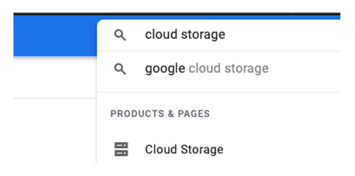
After logging in, you will see the Cloud Console homepage with summarised information. We search for Cloud Storage in the top search bar and select the first service 'Cloud Storage', which takes us to the Cloud Storage Browser.
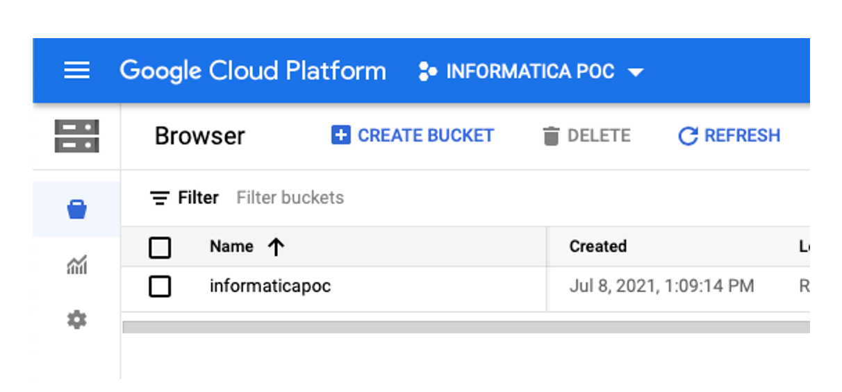
Here we see the informaticapoc bucket, which contains test data.
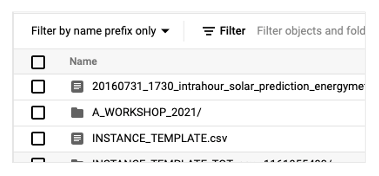
By clicking on the bucket, you can see the contents, including the folder A_WORKSHOP_2021, which we then open.
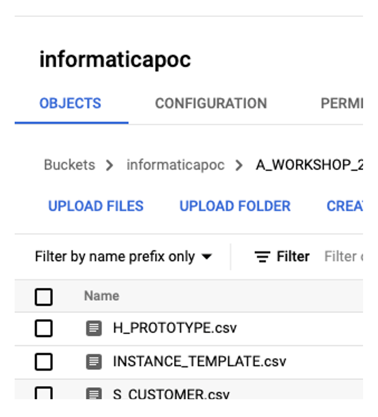
It contains several CSV files. Initially, only the file H_PROTOTYPE.csv is of interest, which is read in later in the mapping.
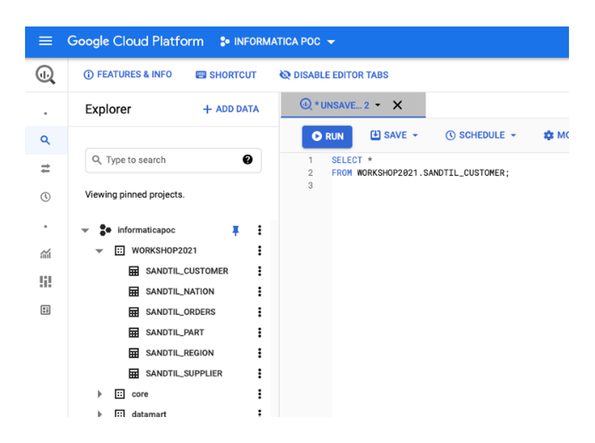
Now we switch to Google BigQuery. Open the side menu (three stripes) and scroll down to the 'Big Data' section and select the BigQuery service. You will now see the BigQuery web frontend. In the sidebar you can see the informaticapoc project and below it various datasets. Only the WORKSHOP2021 dataset is of interest to us. We now create the following table in the editor of the main area:
CREATE TABLE WORKSHOP2021.EXAMPLE_NAME_TEMPLATE(
BK STRING(255),
UTS TIMESTAMP,
CSV_SRC_AND_TGT_FIELD STRING(255),
ORA_SRC_AND_TGT_FIELD STRING(255),
HASH_VALUE STRING(50)
);
Step 2: Log in to Informatica Cloud
Now open a new browser tab and log in to the Informatica Cloud at https://dm-em.informaticacloud.com/ma/home.
You also received an invitation for this in advance. After logging in, you will first see various tiles with the available services. We select Data Integration and go to the homepage. In the menu bar on the left-hand side, click on Explore (the labelling may be in German, depending on your browser settings). We then open the INTF project and search for the folder with the name of our individual employee abbreviation.
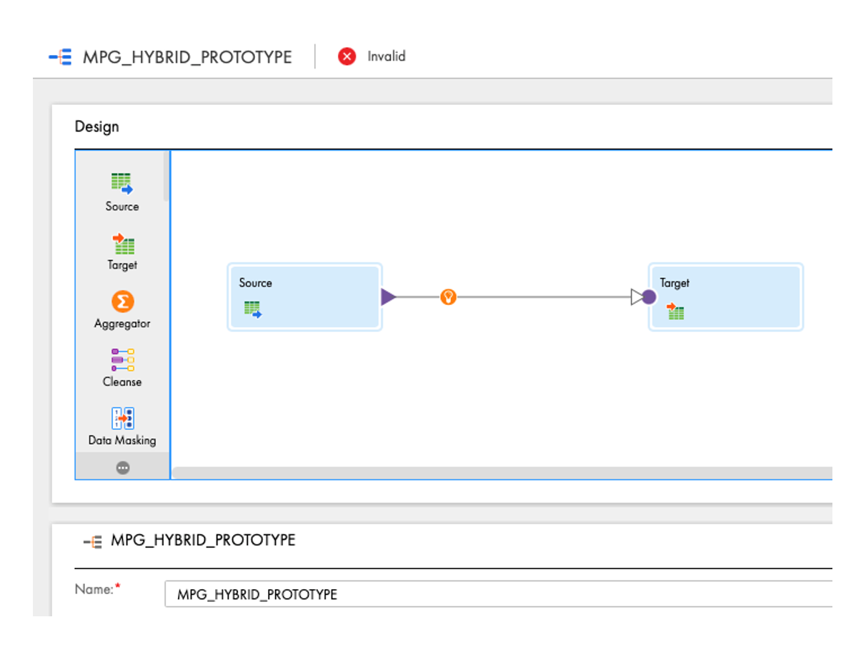
Once you have opened the folder, you will see that there are no objects in it. We now want to change this. In the menu bar, select New... and then under Mappings > Mapping. The Mapping Editor opens, which contains a source-target mapping by default. The result looks like the screenshot on the right. We will now expand this mapping so that we end up joining a CSV file from the storage with data from an Oracle table, calculate a hash value, perform a zero check on certain columns and write the results away in BigQuery.
Step 3: Creation of a mapping
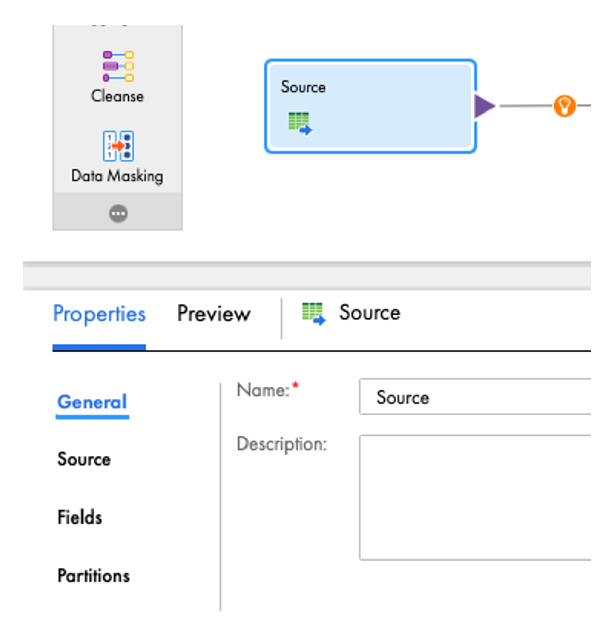
Firstly, we customise the source by clicking on it. The properties of the source open in the lower area. Under General, we assign the name SRC_GCS_CSV for the source and then switch to the Source area, where we select the connection GOOGLE_CLOUD_STORAGE_V2 under Connection.
This connection has been configured in advance in the admin area and refers to the Google Storage bucket opened earlier.
Under Object > Select... we select the file /A_WORKSHOP_2021/H_PROTOTYPE.csv. Now select ‘Delimited’ under Format. To ensure that the file is parsed correctly, we need to select a semicolon as the delimiter under Formatting options. The columns of the CSV file now appear under Fields.
Next, we configure the target. After we have renamed it to TGT_BQ_RESULT, we select the connection GOOGLE_CLOUD_BIG_QUERY_V2 in the Target area under Connection, which refers to our BigQuery project. Under Object > Select... we select the template table EXAMPLE_NAME_TEMPLATE in the WORKSHOP2021 dataset, which we had previously created.
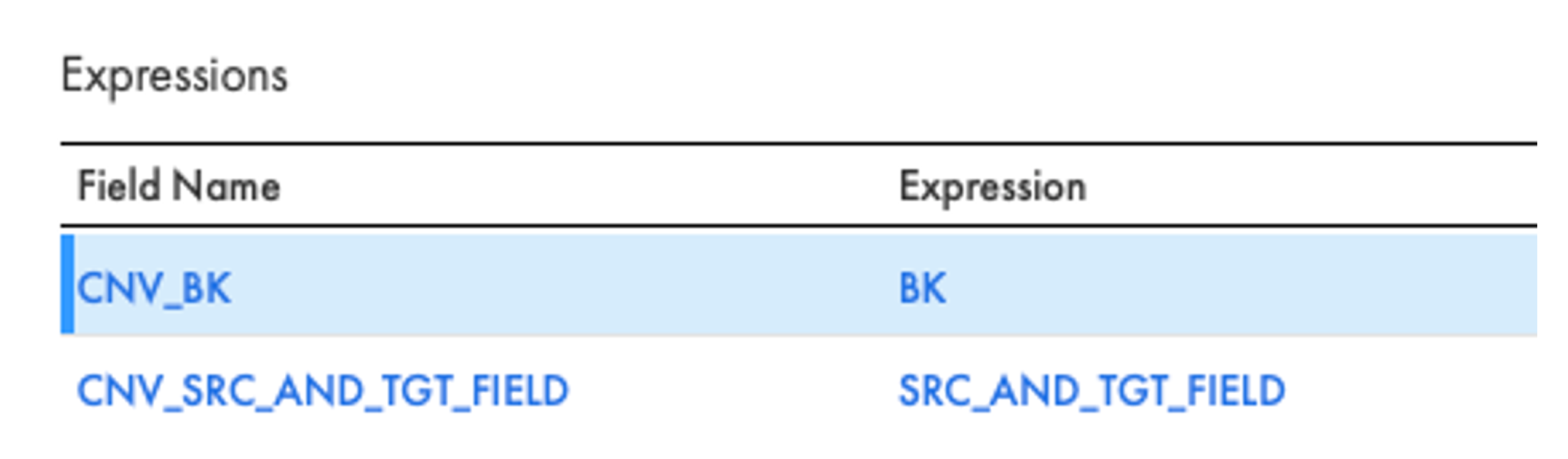
To convert the values from the CSV file, we insert the EXP_CNV_TYPES expression between the source and target by dragging it from the left-hand transformation list onto the connection between the source and target. Under the transformation properties, we add an output field with the name CNV_BK (data type String(50)) in the Expression area. Under Configure... the expression editor opens, in which we first enter the expression BK. Now please save the mapping once. Analogue to the last field, we add an output field with the name CNV_ SRC_AND_TGT_FIELD and the expression SRC_AND_TGT_FIELD. The expression then looks like this:
Next, we create an Oracle source with the name SRC_ORC. We select the connection WSV-DB-01-Playground. Under 'Source Type' we set 'Query'. Now you can define an SQL query under Edit Query.... This construct is known from PowerCenter as a source qualifier, which no longer exists in Informatica Cloud. The following is entered as a query:
SELECT
BK
, UTS
, SRC_AND_TGT_FIELD
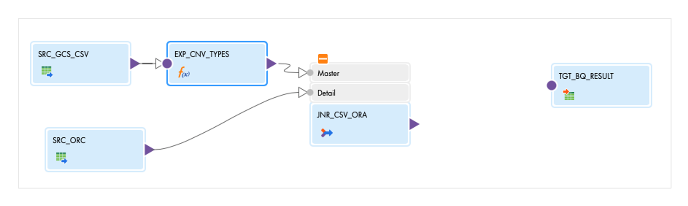
FROM HP_SOURCENow we need to join the Oracle data with the CSV data. To do this, we delete the connection between the expression and the target and add a joiner with the name JNR_CSV_ORA to the mapping. If you click on the orange +, the input groups of the joiner open. We plug the connection from the expression into the master group by dragging the purple arrow of the expression onto the master group. We load the data from the Oracle table into the detail group so that the mapping then looks like this:
In the Joiner, we must now first configure which fields are to be included from the sources. To do this, open the Incoming Fields area in the properties. Here you can define so-called 'Include rules' for the master and detail groups, which control which fields are to be included with which renaming. For the master, we switch to under 'Field Selection Criteria' from 'All Fields' to 'Named Fields'. Then click on Configure... and select only the two fields with the prefix CNV_. In the 'Rename Fields' tab, rename the fields: CNV_BK to CSV_BK and do the same for the other field. Then close the editor with OK. In the detail group we click on Rename... and select 'Prefix' as the Bulk Rename option. Enter 'ORA_' in the text field. Now only the join condition needs to be specified for the joiner. We select CSV_BK = ORA_BK.
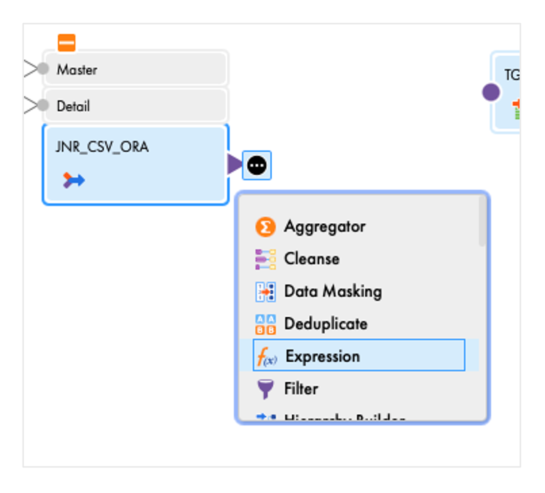
We now attach an expression with the name EXP_PREP_RESULT to the joiner by selecting the joiner and then selecting Expression in the context menu.
We add two output fields:
- VALID_IND, Integer, Expression=1
- HASH_VALUE, String(50), Expression = MD5( CSV_SRC_AND_TGT_FIELD
|| '#'
|| ORA_SRC_AND_TGT_FIELD
)
Note: You must save once after creating each expression.
After the expression, we add a FIL_VALID filter with the filter condition VALID_IND = 1. We then connect the filter to the target.
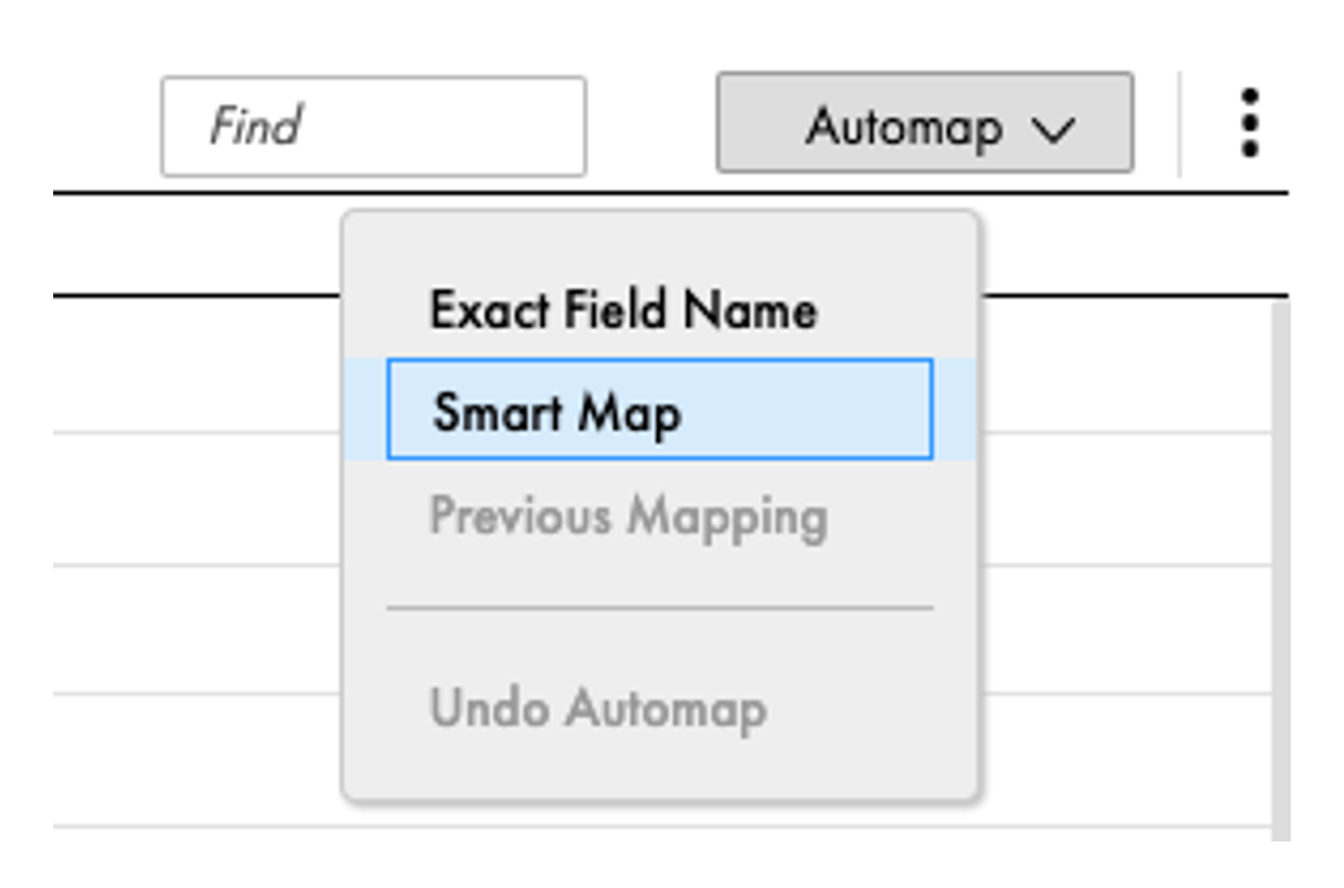
In the target, we still have to map the incoming fields to the fields of the target. To do this, click on the Field Mapping area in the target properties, then on Automap and then on Smart Map. Informatica then maps the fields according to name similarity.
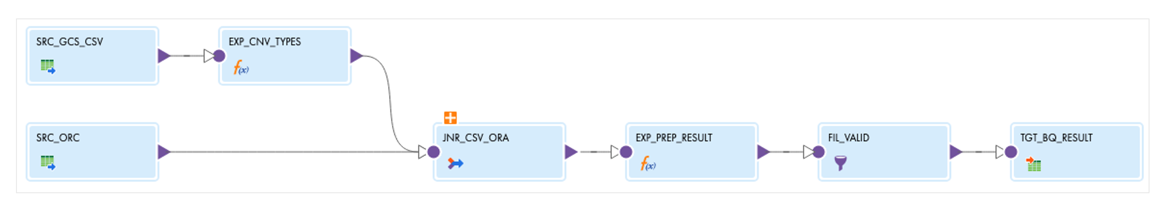
We save the mapping. It should be in the valid state after validation. It looks like this:
Step 4: Creation of a mapping task and taskflow
In the left bar, click New... and then create a mapping task with the name TSK_HYBRID_PROTOTYPE. We select intf-local-linux as the runtime environment. This environment is an Informatica Secure Agent, which is installed in the Frankfurt office.
We select the mapping we have just created as the mapping and then click Finish.
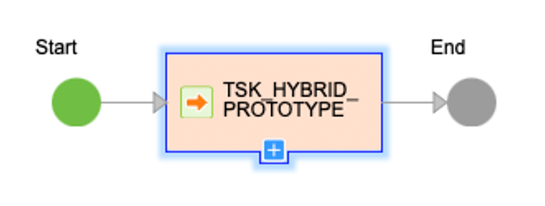
Finally, we create a taskflow under New... > Taskflows > Taskflow. We name this WFL_HYBRID_PROTOTYPE. Between Start and End, we drag a Data Task from the bar and name it TSK_HYBRID_PROTOTYPE. In the Data Task area, we must select the mapping task we have just created. To do this, click on Select and then on Explore > Projects and Folders at the top left of the window and then navigate to /INTF/EXAMPLE_NAME. Select the mapping task there.
Now save the taskflow.
Step 5: Testing the taskflow
We would now like to test the taskflow we have just created. To do this, we go to our folder under Explore and right-click to open the context menu of the taskflow, where we select Run. Now we switch to the My Jobs area in the left bar. The first line there shows the job that has just been started. We wait for the result of the taskflow. This should end with the status Success. Under View Subtasks you can see the mapping task and in the Rows Processed line there should be a 1, i.e. exactly one row should be written to the target.
In the BigQuery frontend we open the table EXAMPLE_NAME_TEMPLATE and under Preview we should see the following result:

Step 6: Log in to MetaKraftwerk
Now that we have successfully built a prototype, we would like to develop it further as a pattern. To do this, we log into MetaKraftwerk at https://app.metakraftwerk.com/. Account information was sent in advance by email.

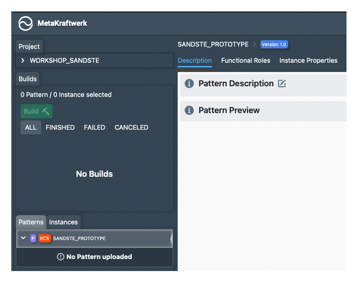
We switch to the WORKSHOP_EXAMPLE_NAME project via the menu bar. There you can see the project, the previous builds (none available) and the pattern EXAMPLE_NAME_PROTOTYPE, which is now to be created, in the left-hand bar. If we click on the pattern, we will see various tabs in the main area (Description, Functional Roles, ...).
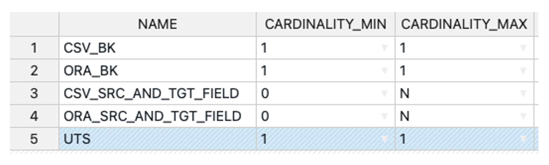
We start by creating the following functional roles (pay attention to the cardinalities!):
We do not need to create instance properties, the standard set is sufficient: UNCTIONAL_ROLE, NAME, DATA_TYPE, PRECISION, SCALE, NULLABLE.
We now import the template previously created in Informatica into our pattern by clicking on 'Fetch Pattern' at the top right, then on 'Connect' and then in our folder /INTF/EXAMPLE_NAME folder and then select the taskflow. The import starts with 'Fetch 1 Object', which we only have to confirm at the end with 'Commit Upload'.
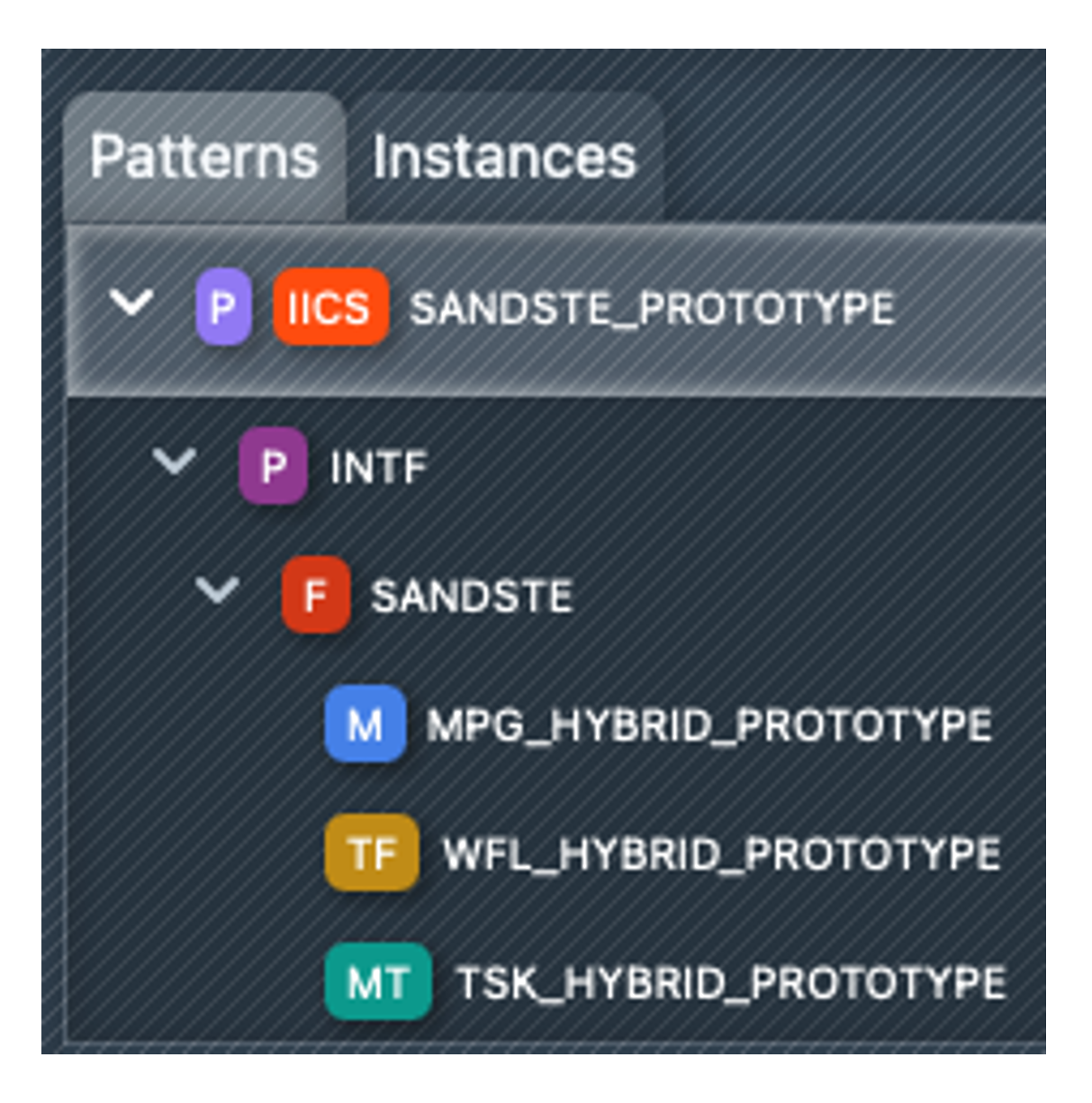
You will then see the pattern objects on the left in the pattern browser (see screenshot on the right). As you have selected the taskflow, the dependencies (mapping task and mapping) are also imported automatically.
If you click on the mapping, it opens in the pattern editor.
What is still missing are rules on how to create executable process instances from the template. To do this, we need to make dynamic configurations at various points in the mapping, e.g:
- Naming rules for mapping, task and taskflow
- Table names
- Fields incl. data types for sources and targets
- Expressions
- Join and filter conditions.
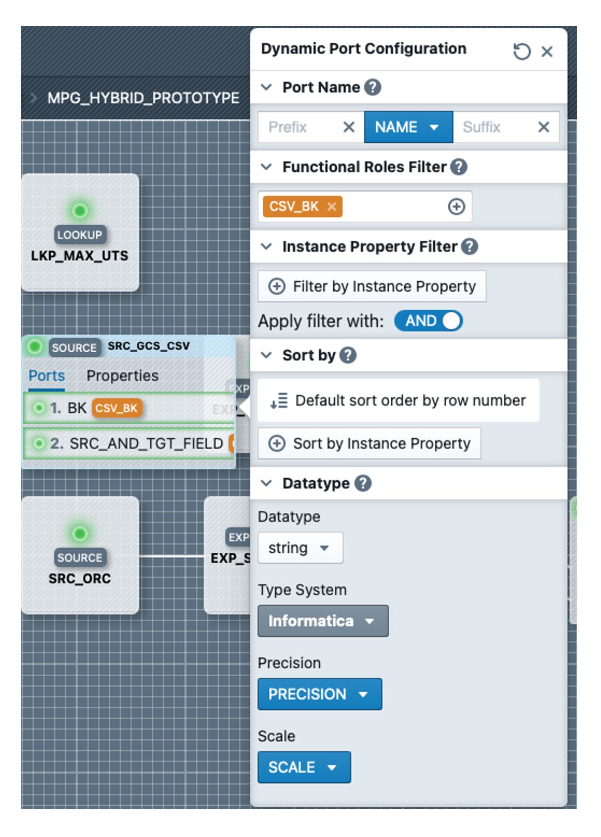
We start with the source SRC_GCS_CSV, open it by double-clicking and open the port editor by clicking on the port BK. In the editor we select CSV_BK as the functional role, under Datatype in the dropdown 'string' as Fixed Value, and as Type System Informatica. The result should look like the screenshot on the right. We make the settings for the SRC_AND_TGT_FIELD field in the same way, except that we select the CSV_SRC_AND_TGT_FIELD role here.
Now we switch to the properties in the source and open the editor by clicking on the 'Object / Table Name' property. By activating the 'Advanced Configuration' tick box, we can define a complex expression. We content ourselves with replacing H_PROTOTYPE with S__csv and then dragging and dropping the INSTANCE_NAME from the 'References' area after S_ so that the result looks like this:
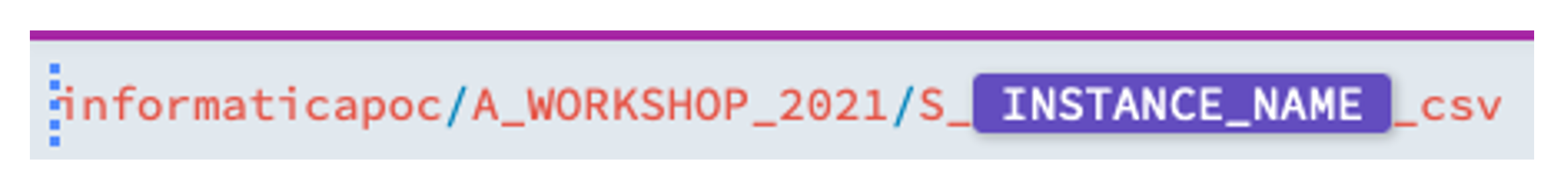
Where the placeholder INSTANCE_NAME is located, the respective instance name is later inserted in an instance. We are finished with the source.
Next, we configure the SRC_ORC source. There we have to configure the three ports BK, UTS and SRC_AND_TGT_FIELD again and assign the functional roles ORA_BK, UTS and ORA_SRC_AND_TGT_FIELD to them. We leave the remaining settings in the port editor with the defaults this time.
In the Source-Properties, we still have to adjust the query of the source (Tip:The query property of a source is analogous to a Source Qualifier SQL query in PowerCenter).
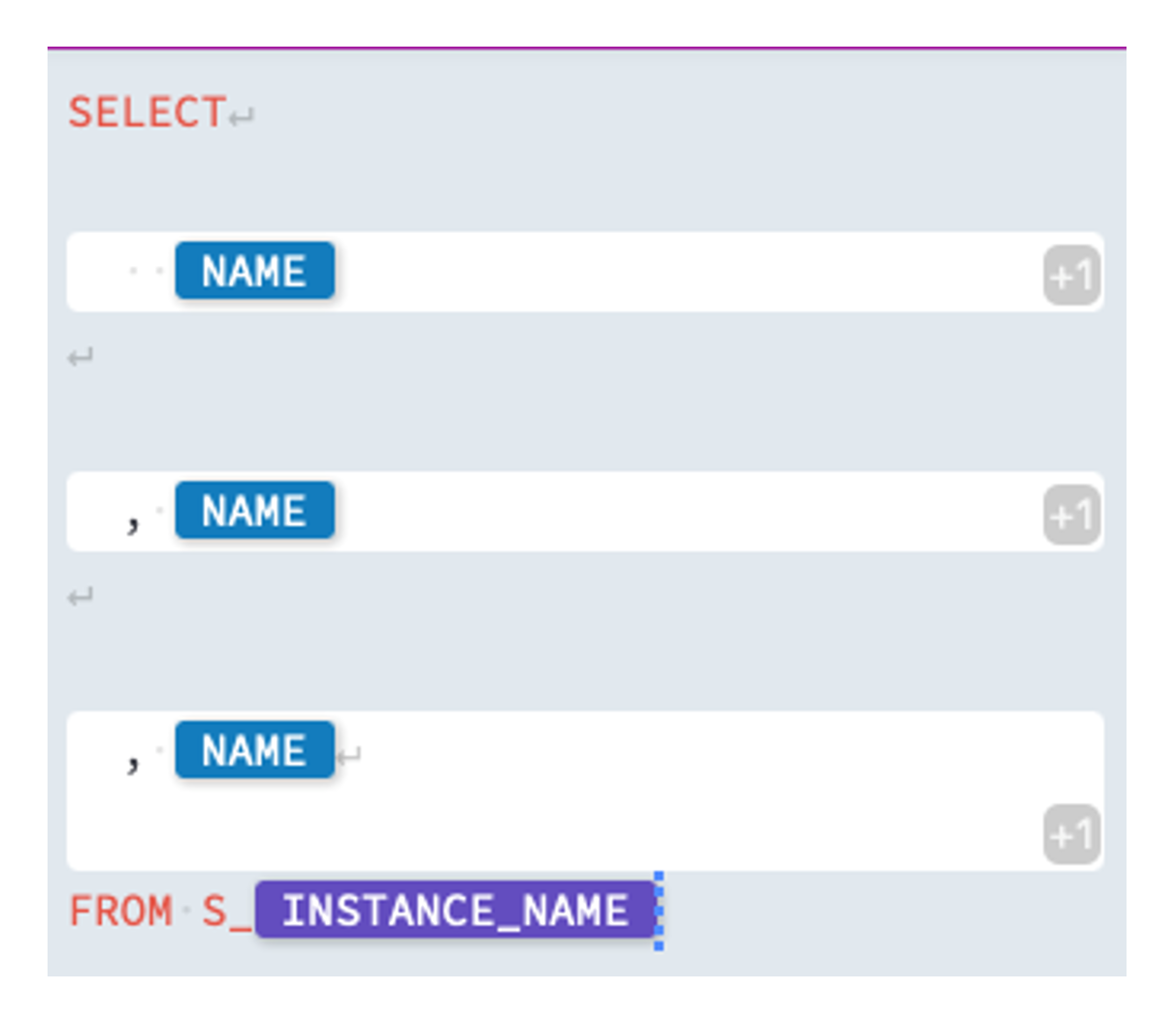
By opening the Advanced Editor of the properties again, we can create a dynamic SQL template, which should look like the screenshot on the right. The aim is to select the Business-Key, the Update-Timestamp and the Source-And Target-Fields.
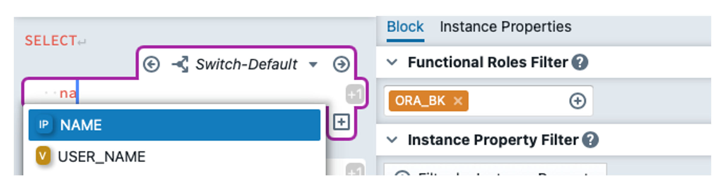
We first delete everything except for the first line. Then click on ![]() to create a new expression block. An expression block makes it possible to access instance metadata by defining which functional roles are used (and optionally other filter criteria). In the block itself, you can then use instance properties as placeholders for specific metadata values. We start by selecting the functional role ORA_BK for the block we have just created and using NAME as the instance property. This is done by typing 'na' in the block and then selecting the instance property with the auto-complete, or via the 'Instance Properties' tab, where you can drag and drop it into the block. Our block is now ready.
to create a new expression block. An expression block makes it possible to access instance metadata by defining which functional roles are used (and optionally other filter criteria). In the block itself, you can then use instance properties as placeholders for specific metadata values. We start by selecting the functional role ORA_BK for the block we have just created and using NAME as the instance property. This is done by typing 'na' in the block and then selecting the instance property with the auto-complete, or via the 'Instance Properties' tab, where you can drag and drop it into the block. Our block is now ready.
To display the previous result, you can select the instance TEST_INSTANCE at the top right under 'Preview Instance'. If you then open the property editor for the query again, the editor has split and on the right-hand side you can now see what the query for the TEST_INSTANCE would look like.
We now create another block similar to the first one, but this time we select UTS as the functional role.

This time we add a comma before the NAME.
Now we copy the second block by selecting it using the known text selection and then copying it with Ctrl+C. Then move the cursor all the way down and paste the block using Ctrl+V. In this third block, we change the functional role to ORA_SRC_AND_TGT_FIELD and insert a line break in the block.
After the block, we add  the instance name from the references or enter it via auto-complete. The template should now look like the screenshot above.
In the next step, we need to convert the values read from the CSV file to the correct data type. There is nothing to do for strings, but decimal values must be converted using TO_DECIMAL. We open the EXP_CNV_TYPES transformation and click on the CNV_BK field. In the expression editor, we switch off the 'Aggregate Fields' checkbox. For the expression name, we enter the prefix CNV_ and leave the instance property NAME.
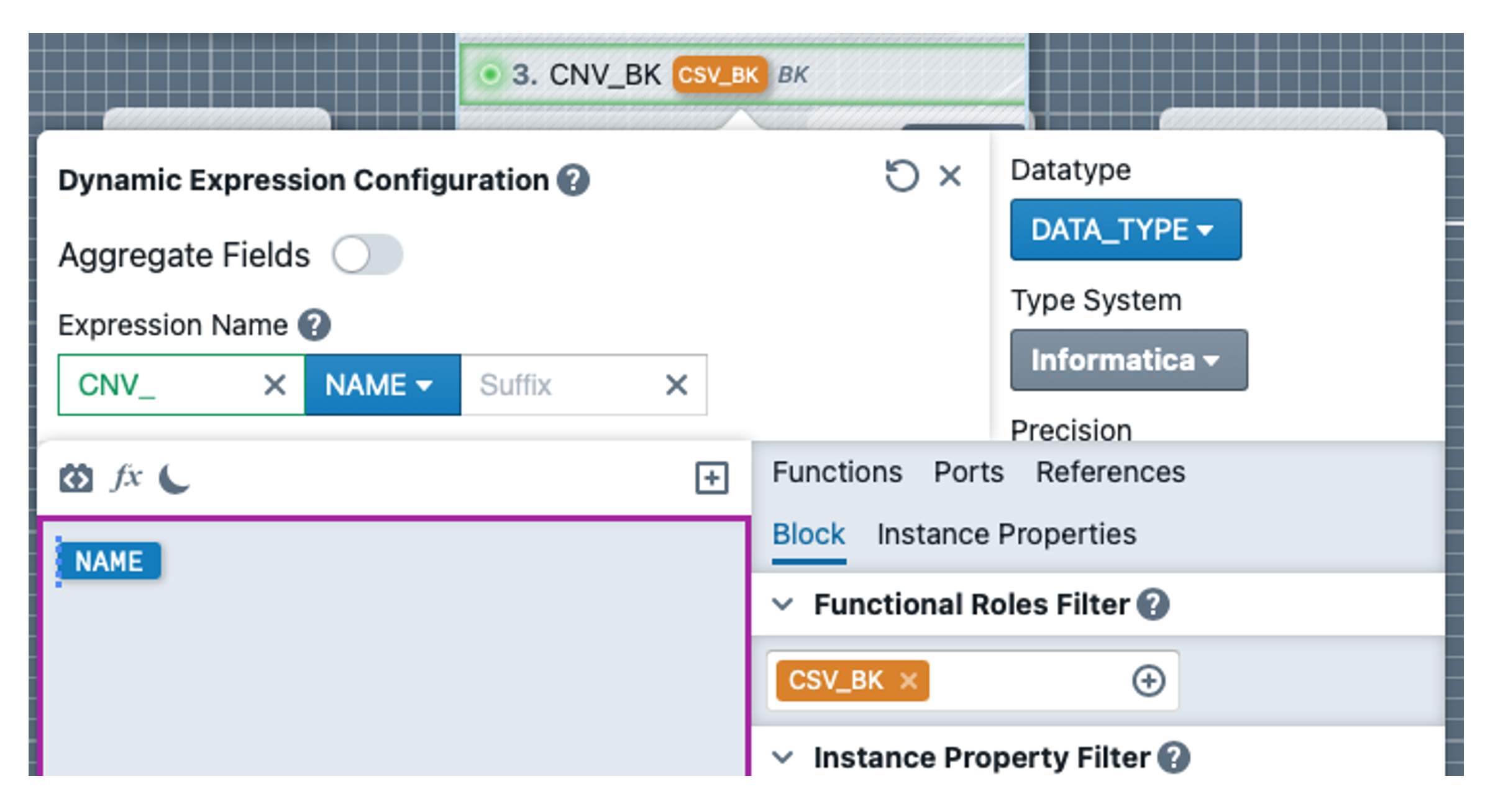
In the text editor, we also add the instance property NAME so that the value from the CSV source is simply used for the default case. In the Functional Roles Filter of the block, we select the role CSV_BK. The result can be seen in the screenshot on the right.
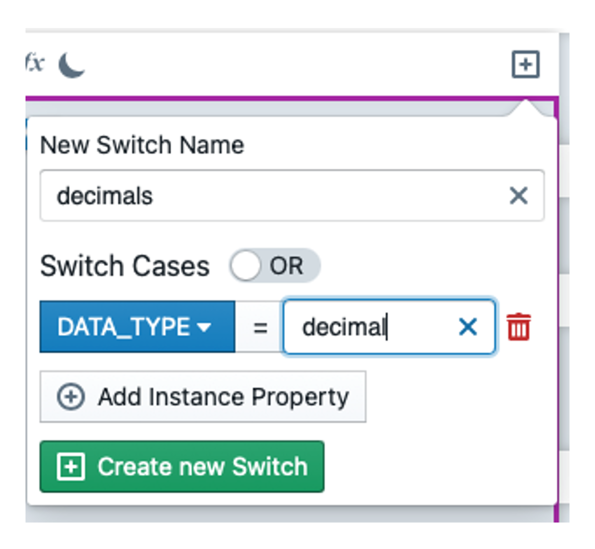
Now we define the case that the BK is of type decimal. To do this, we click on ![]() so that a popover for a new expression switch opens. We enter decimals as the name and insert a switch case with DATA_TYPE = decimal. We confirm with 'Create new Switch'.
so that a popover for a new expression switch opens. We enter decimals as the name and insert a switch case with DATA_TYPE = decimal. We confirm with 'Create new Switch'.
The text editor is now empty again and we enter the expression  .
.
We define the CNV_SRC_AND_TGT_FIELD in the same way as the CNV_BK.
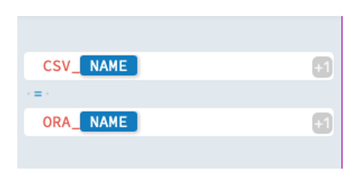
Now we will adapt the join condition of the JNR_CSV_ORA joiner by opening the transformation and editing the 'Join Condition' property under Properties in Advanced mode. We insert two expression blocks there separated by ' = '. We select the functional roles CSV_BK and ORA_BK for the blocks. We write CSV_NAME or ORA_NAME in the blocks so that the expression looks like the screenshot on the right.
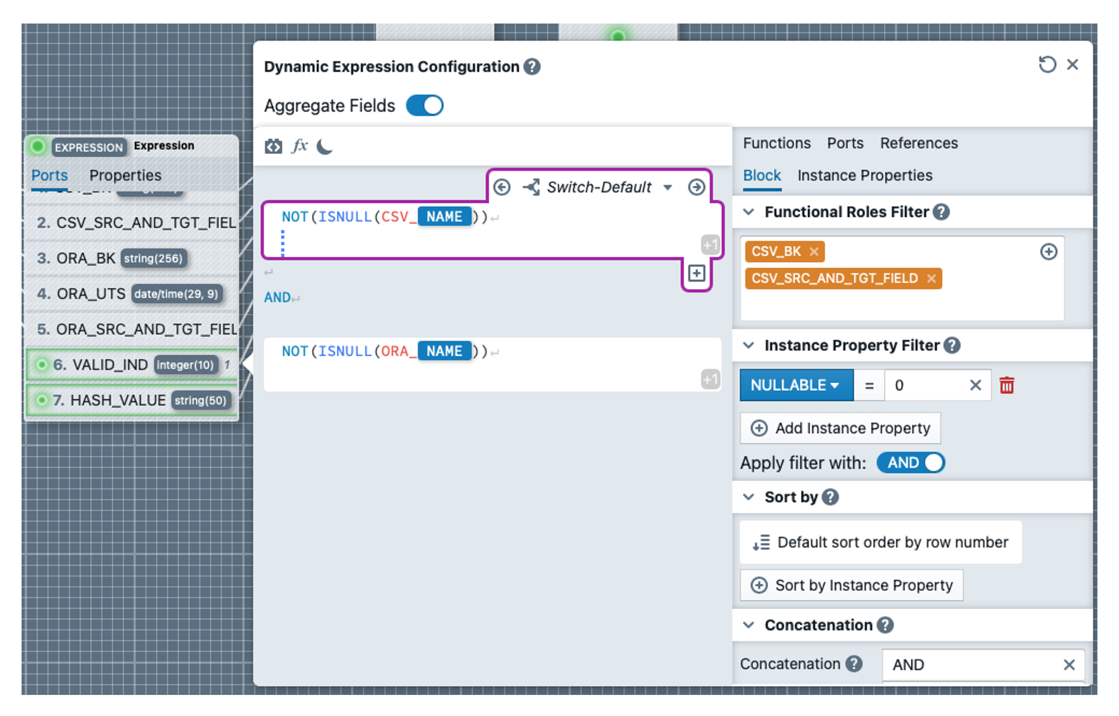
In the EXP_PREP_RESULT transformation, we still have to define two dynamic expressions. To do this, we first click on VALID_IND, delete the 1 and add an expression block (note: the 'Aggregate Fields' switch remains activated this time). In this we write the expression NOT(ISNULL(CSV_NAME))(incl. line break). We select the roles CSV_BK and CSV_SRC_AND_TGT_FIELD for the block. We also add the condition NULLABLE = 0 under Instance Property Filter. Further down under Concatenation we add ' AND ' as Concatenation for the block. By clicking on the 'Switch-Default' tab, a dropdown opens and we can switch to 'Block-Default', where we enter TRUE. We copy the entire block again and paste it at the bottom. We change the roles in the second block and select ORA_BK and ORA_SRC_AND_TGT_FIELD.
We write an AND between the blocks. In the expression, we replace CSV_ with ORA_ The result should look like the screenshot below:
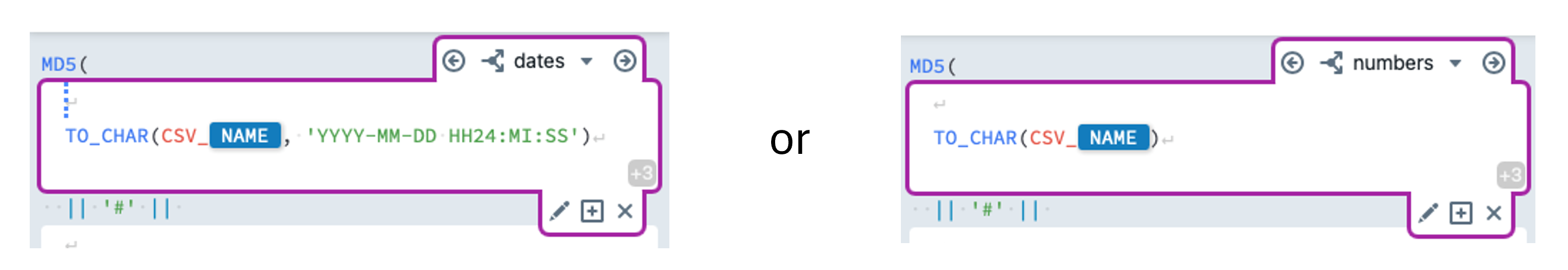
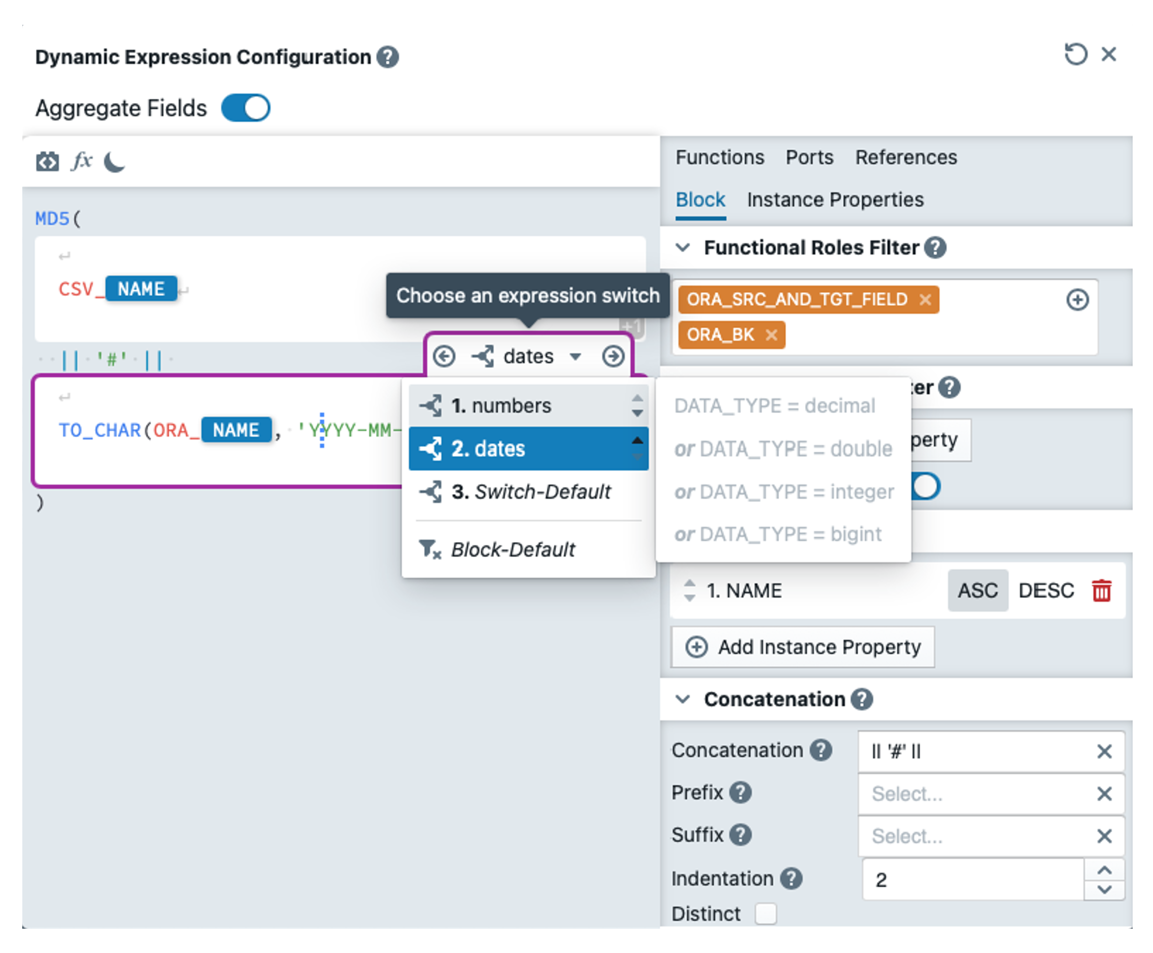
Now we define the last expression HASH_VALUE. We delete everything except MD5() and insert a block in the brackets in which we write CSV_NAME. We set the functional roles to CSV_BK and CSV_SRC_AND_TGT_FIELD. In the block properties, we set the sequence to the instance property NAME (Ascending) under 'Sort By'. We enter "|| '#' ||" as the Concatenation and a little further down we set the Indentation to 2. "'#'" must also be entered in the block default switch (only with single inverted commas). We need to perform a string conversion for numeric and date values. To do this, we insert two switches in the block, which are defined as follows:
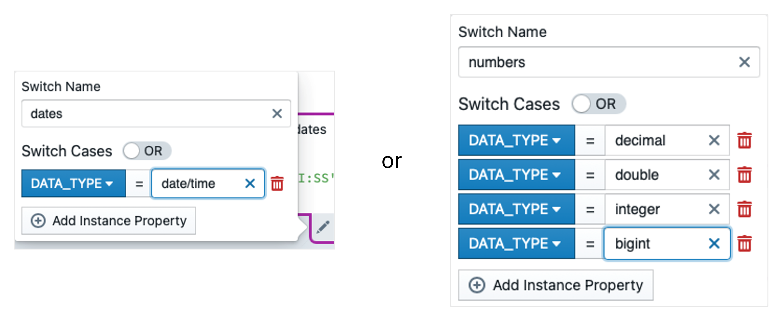
We insert the following expressions into these switches:
We again copy the entire block under the first one and replace the roles with ORA_BK and ORA_SRC_AND_TGT_FIELD. In the block, we replace the prefix CSV_ in all switches with ORA_. We insert "|| '#' ||" between the blocks so that the values of both blocks are concatenated correctly. The result is shown in the following screenshot:
Last but not least, the target needs to be customised. We want to define the table name of the target as a reusable expression. To do this, we click on the pattern on the left and then on the 'Reusable Expressions' tab at the top. There we create a new expression with the name TARGET_NAME by clicking on ![]() . We insert the following expression into this:
. We insert the following expression into this:  . USER_NAME is a pattern variable whose value can be changed in the 'Variables' tab, but we leave this value as our abbreviation. We switch back to the mapping and open the TGT_BQ_RESULT target and the 'Object / Table Name' property there. We insert the expression
  there (in Advanced mode).
So that MetaKraftwerk knows what the mappings, tasks and taskflows to be created should be called, we need to define naming rules for these three objects. To do this, we click on the EXAMPLE_NAME folder in the left-hand bar. Then we first click on the mapping so that its name editor opens. Under Default Name, we enter MPG_ as the prefix. Similarly, we enter the prefix TSK_ for the task and the prefix WFL_ for the taskflow.
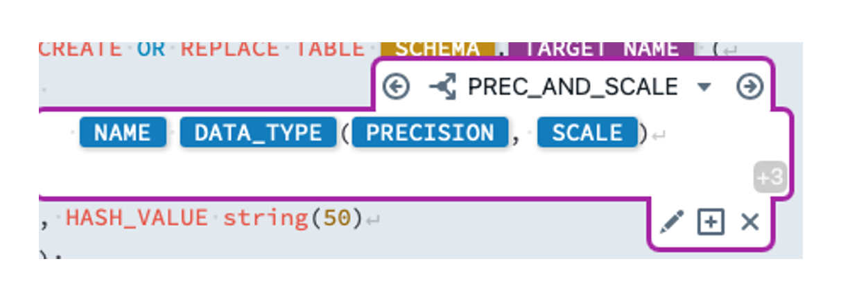
In order to actually run the mappings, the target tables still need to be created in BigQuery. As we don't want to type the DDLs ourselves, we create a DDL template with MetaKraftwerk. To do this, we click on the Pattern and then on the 'Files' tab. There we create a new file with the name 'CREATE_BIGQUERY_TABLE_DDLs.sql' by clicking on ![]() . We select 'Google Big Query V2' as the format for the file at the top of the header. In the text editor, we enter the template below (screenshot), where SCHEMA is again a pattern variable and TARGET_NAME is a reusable expression (to be found under References). For the functional roles, we select the roles CSV_BK, CSV_SRC_AND_TGT_FIELD, ORA_SRC_AND_TGT_FIELD and UTS. ORA_BK is omitted as it would be redundant to CSV_BK. We specify a comma as the concatenation.
. We select 'Google Big Query V2' as the format for the file at the top of the header. In the text editor, we enter the template below (screenshot), where SCHEMA is again a pattern variable and TARGET_NAME is a reusable expression (to be found under References). For the functional roles, we select the roles CSV_BK, CSV_SRC_AND_TGT_FIELD, ORA_SRC_AND_TGT_FIELD and UTS. ORA_BK is omitted as it would be redundant to CSV_BK. We specify a comma as the concatenation.
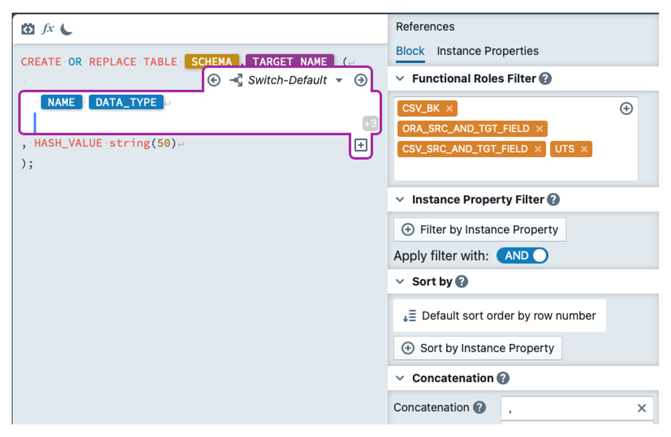
We first enter the default switch  . Then we create another switch with the following configuration:
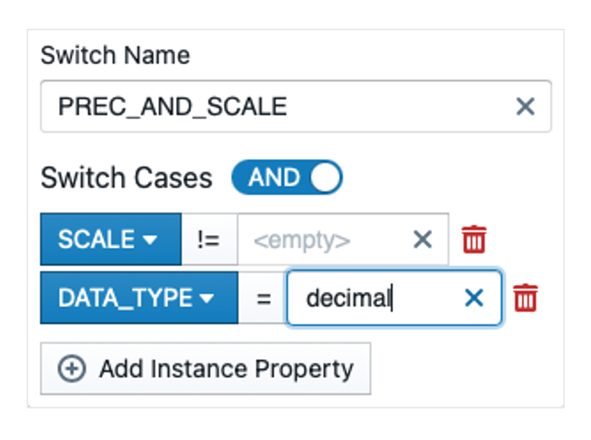
It is particularly important to ensure that the tick is changed from  to
to  and that Scale != is empty. The operator can be changed by clicking on ' = '. We enter the following expression in the switch:
Now we add the following switch:
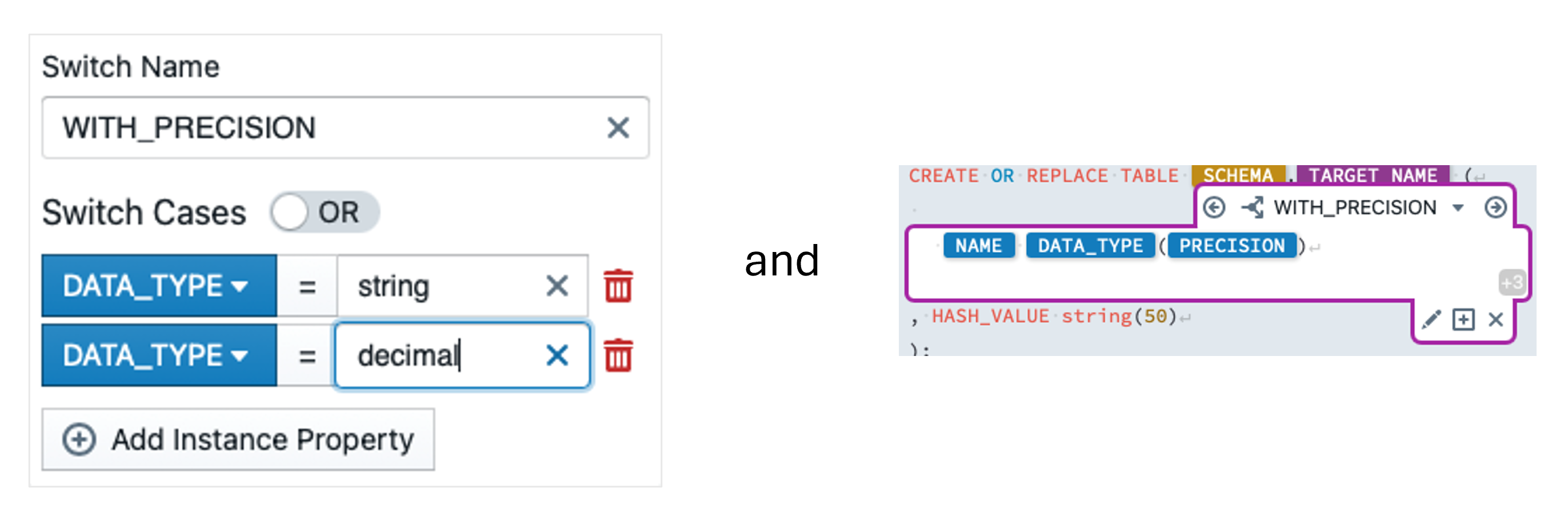
Now our pattern is complete.
Step 7: Build & Deployment
In order to create executable instances for Informatica from the pattern, we need instance metadata. You have received this in the email as XLSX. In the left bar, we now switch to the 'Instances' tab. At the bottom we click on 'Import metadata file... (xlsx, xlsm) Browse' and select the Excel WORKSHOP_INSTANCES_EXAMPLE_NAME.xlsx. The instances now appear below the pattern. The CUSTOMER instance is labelled as invalid. We open the instance and rectify the error by setting the precision of the C_CUSTKEY field to 20.
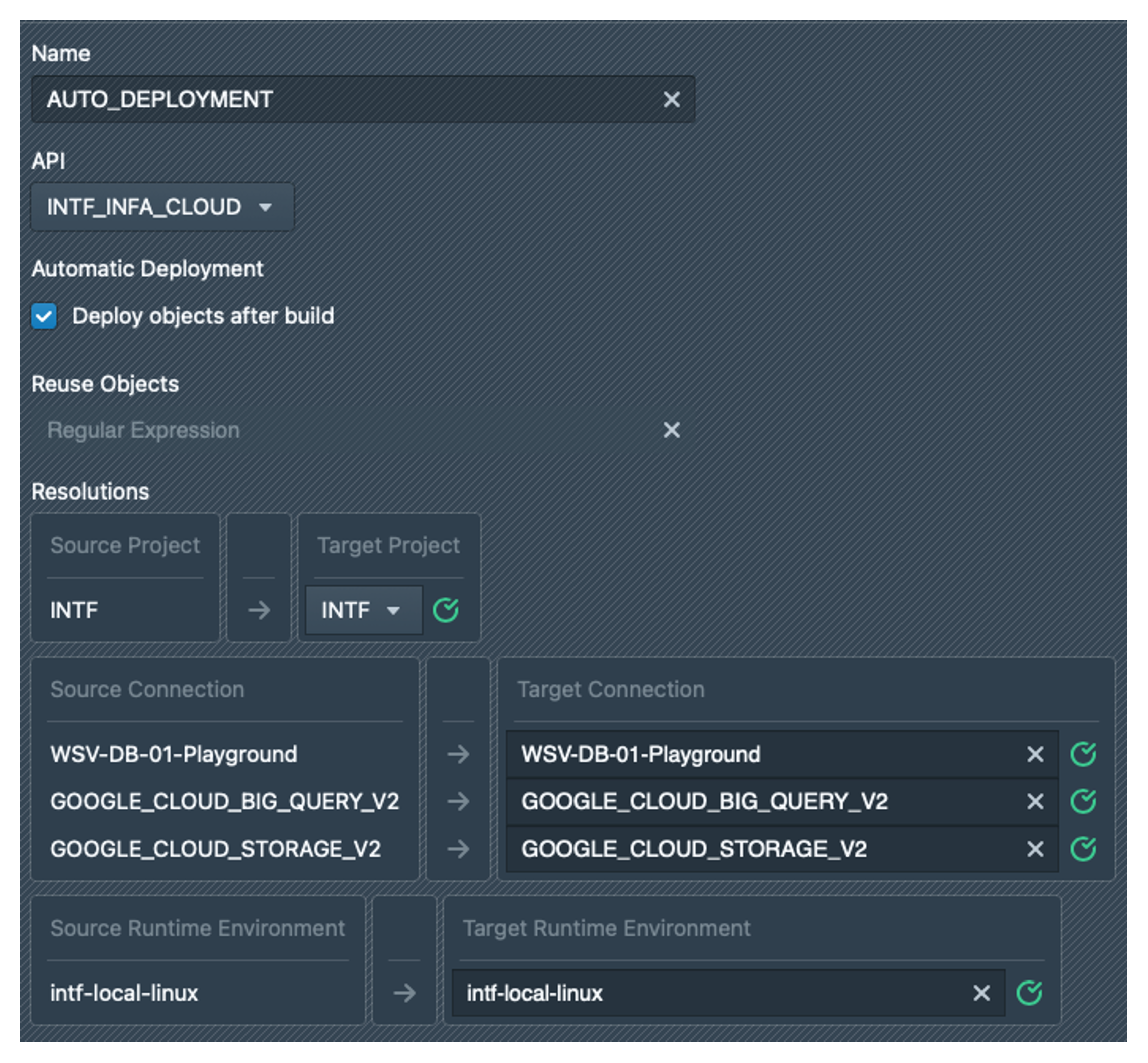
Before we create the instances, we create a deployment configuration. To do this, we click on the pattern again and then on the Deployments tab. Click on ![]() to create a deployment with the name AUTO_DEPLOYMENT. For this configuration, we select the API INTF_INFA_CLOUD and activate the checkbox for Automatic Deployment. Under Resolutions, we select the INTF project as the target project in the dropdown. For the connections and the runtime environment, we always simply select the same value as the source as the target, preferably by copying and pasting. The green tick should always appear, otherwise the specified value was not found in Informatica. The result should look like the screenshot below:
to create a deployment with the name AUTO_DEPLOYMENT. For this configuration, we select the API INTF_INFA_CLOUD and activate the checkbox for Automatic Deployment. Under Resolutions, we select the INTF project as the target project in the dropdown. For the connections and the runtime environment, we always simply select the same value as the source as the target, preferably by copying and pasting. The green tick should always appear, otherwise the specified value was not found in Informatica. The result should look like the screenshot below:
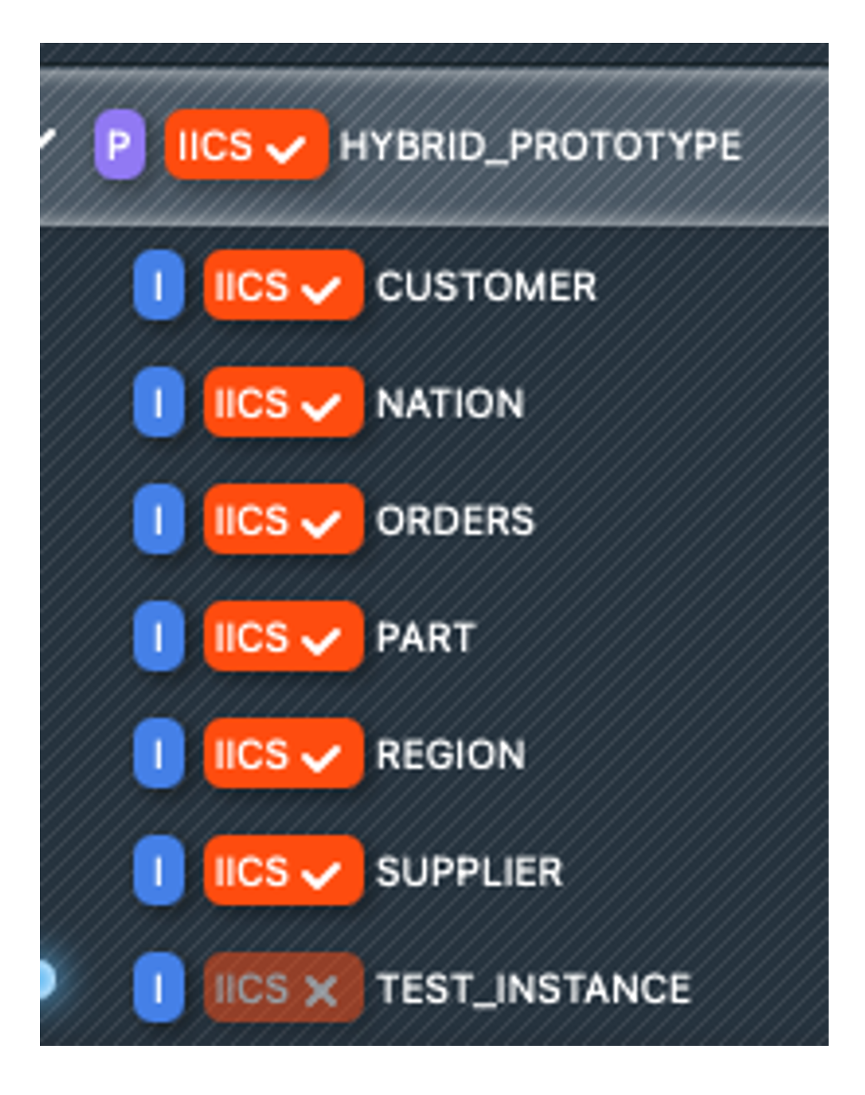
Now we select all instances except for TEST_INSTANCE by clicking on the label  . Now we can click on
  at the top. After a short time, the instances are created and also deployed directly from MetaKraftwerk to our Informatica folder.
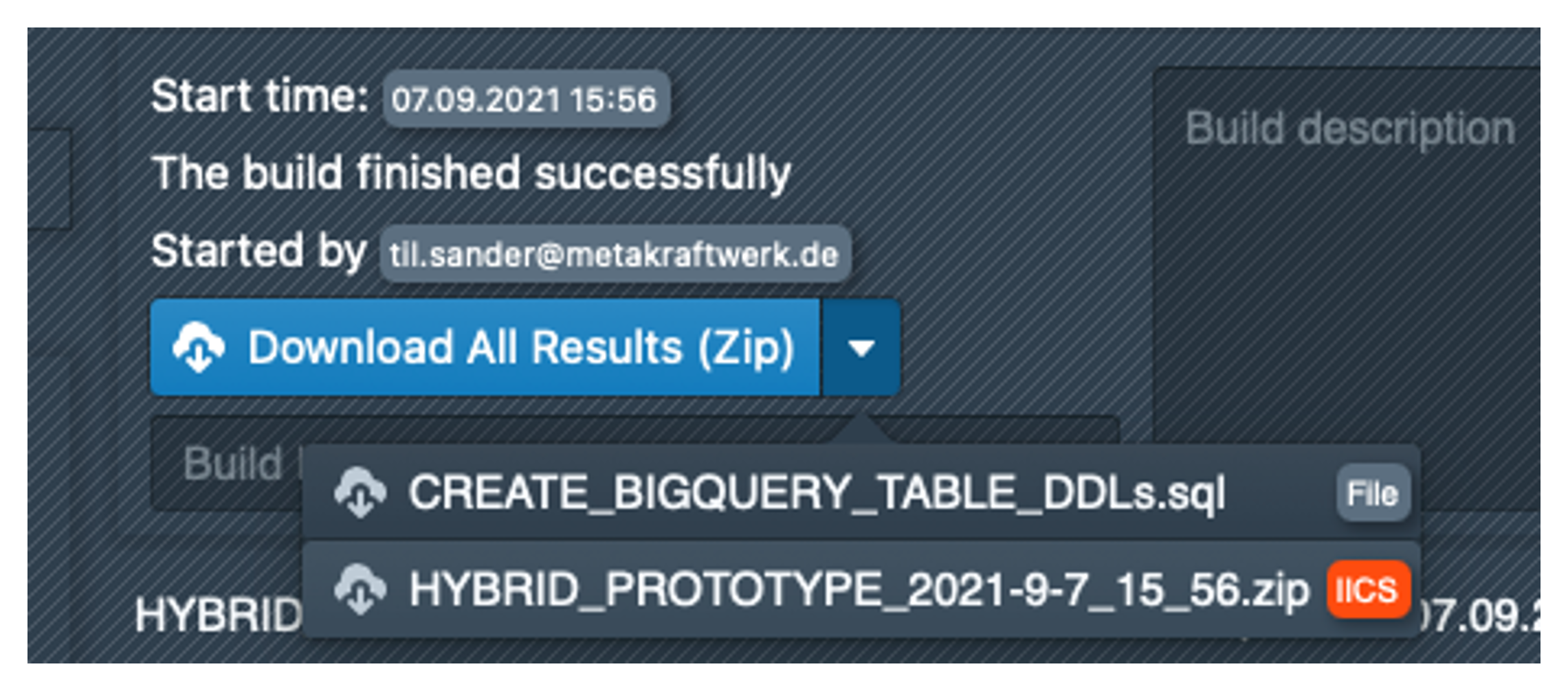
If we click on the last build, it is possible to download the created DDL file by clicking on the check mark next to 'Download All Results (Zip)'.
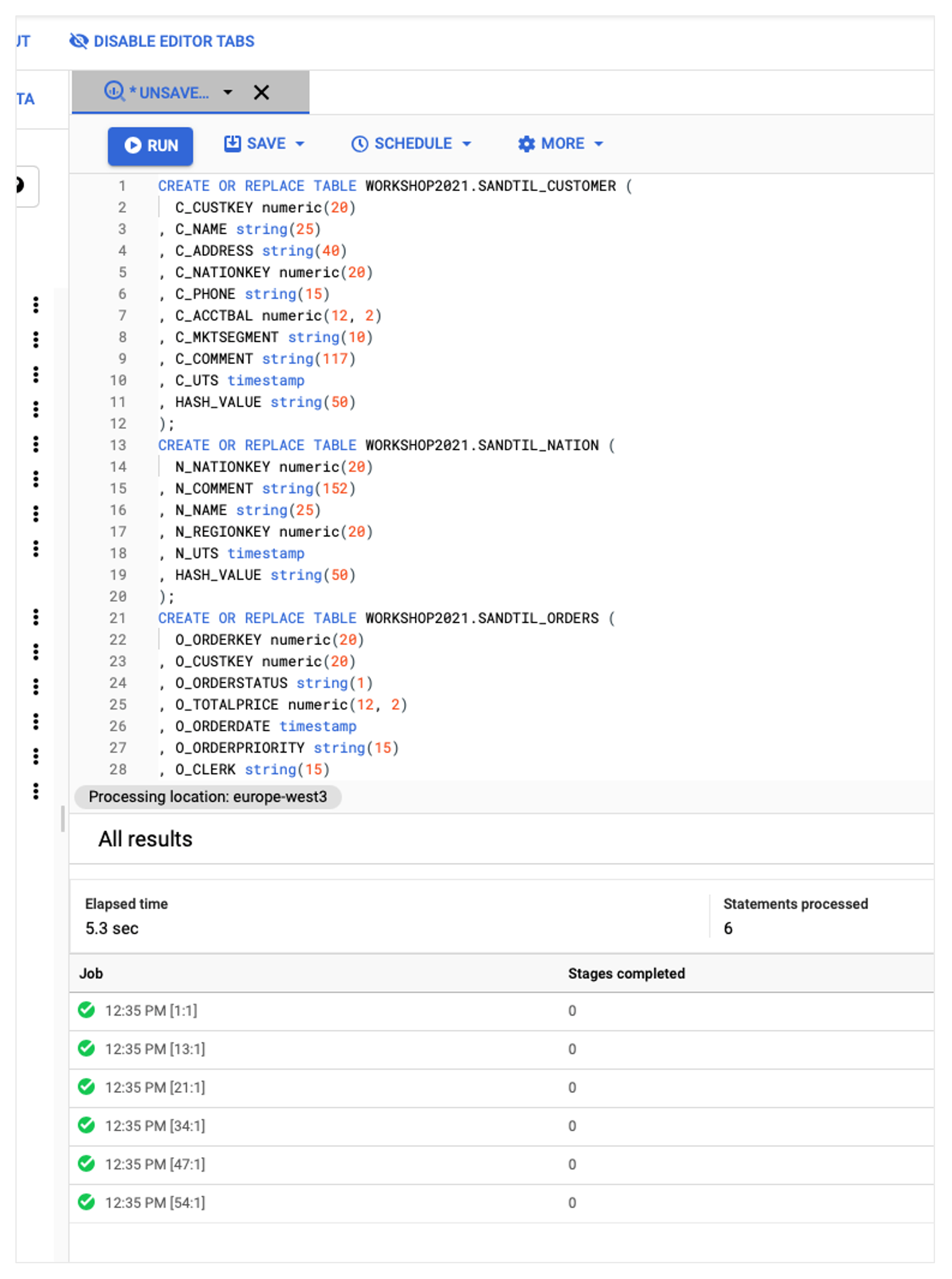
This must be opened in a text editor and the content then inserted into BigQuery. The tables can then be created using Run. BigQuery should execute six successful jobs as shown below.
Now that the table structures are available in BigQuery, we can execute the mappings. To do this, we switch to our folder in the Informatica Cloud, which should now contain six new taskflows. Both the taskflows and the mappings should all be valid. We first start the WFL_CUSTOMER taskflow by right-clicking on it to open the context menu and then clicking on Run. Now we switch to 'My Jobs' in the left bar and see that the taskflow is now running. After a short wait, the job should end with the status 'Success'.
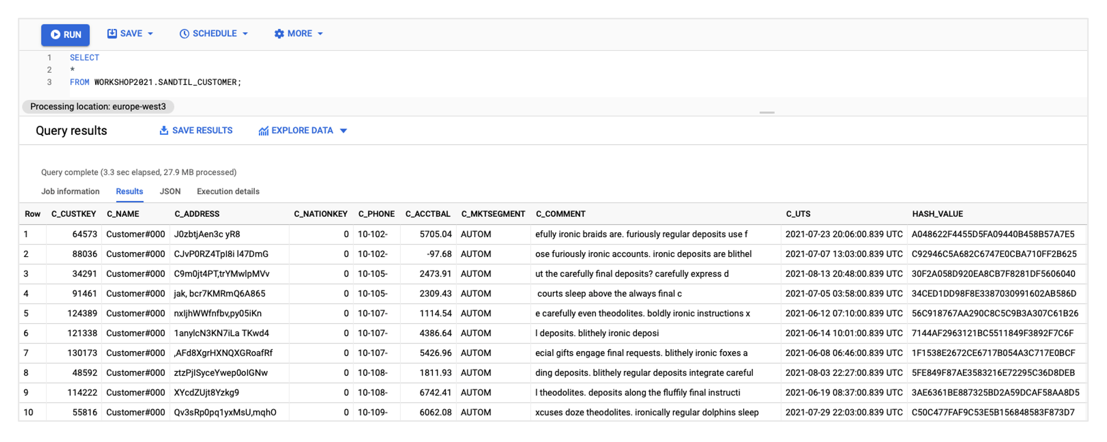
In BigQuery, you can now view the EXAMPLE_NAME_CUSTOMER table, which should be filled with values:
If this has worked, the remaining five taskflows can also be started. To check whether the results are correct, you can run the following query in BigQuery, all instances should be valid:
SELECT 'CUSTOMER' AS INSTANCE, TO_HEX(MD5(STRING_AGG(HASH_VALUE)))='037cba5c79d0bc732572137756933f49' AS IS_VALID FROM (SELECT HASH_VALUE FROM WORKSHOP2021.[EXAMPLE_NAME]_CUSTOMER ORDER BY HASH_VALUE ASC)
UNION ALL
SELECT 'NATION' AS INSTANCE, TO_HEX(MD5(STRING_AGG(HASH_VALUE)))='b0397def9c4b11250fbbcb1b5f00a5de' AS IS_VALID FROM (SELECT HASH_VALUE FROM WORKSHOP2021.[EXAMPLE_NAME]_NATION ORDER BY HASH_VALUE ASC)
UNION ALL
SELECT 'ORDERS' AS INSTANCE, TO_HEX(MD5(STRING_AGG(HASH_VALUE)))='61aa753600720af75da75ff7a31c1b73' AS IS_VALID FROM (SELECT HASH_VALUE FROM WORKSHOP2021.[EXAMPLE_NAME]_ORDERS ORDER BY HASH_VALUE ASC)
UNION ALL
SELECT 'PART' AS INSTANCE, TO_HEX(MD5(STRING_AGG(HASH_VALUE)))='2dfb3ec738fd2093eb269bdae6c6e693' AS IS_VALID FROM (SELECT HASH_VALUE FROM WORKSHOP2021.[EXAMPLE_NAME]_PART ORDER BY HASH_VALUE ASC)
UNION ALL
SELECT 'REGION' AS INSTANCE, TO_HEX(MD5(STRING_AGG(HASH_VALUE)))='ff32093d6d55e83e44e776fa68e5aeb0' AS IS_VALID FROM (SELECT HASH_VALUE FROM WORKSHOP2021.[EXAMPLE_NAME]_REGION ORDER BY HASH_VALUE ASC)
UNION ALL
SELECT 'SUPPLIER' AS INSTANCE, TO_HEX(MD5(STRING_AGG(HASH_VALUE)))='9edbe240d5e1b87d371c3ed0ad8bbd19' AS IS_VALID FROM (SELECT HASH_VALUE FROM WORKSHOP2021.[EXAMPLE_NAME]_SUPPLIER ORDER BY HASH_VALUE ASC)
;
Phase II. Extension with UTS delta mechanism
Now that we have successfully built and executed the pattern, we would like to extend it with a simple delta mechanism. We want to implement a lookup that looks at the target table and then filters out all Oracle source records in the mapping whose UTS is less than or equal to the maximum UTS in BigQuery.
Step 1: Customisation of the prototype in Infa Cloud
We switch back to Informatica and open our mapping MPG_HYBRID_PROTOTYPE. In this, we first add a lookup with the name LKP_MAX_UTS. A field with the name LKP_PARAM must be added to the transformation under Properties > Incoming Fields. Under Lookup Object, we select the connection GOOGLE_CLOUD_BIG_QUERY_V2 and set Source Type to 'Query' in order to define the following query:
SELECT
'X' AS PARAM,
COALESCE(MAX(UTS), TIMESTAMP '9999-12-31 00:00:00.00-00') AS MAX_UTS
FROM WORKSHOP2021.[EXAMPLE_NAME]_TEMPLATE;
PARAM = LKP_PARAM must be selected as the lookup condition. Under Return Fields, MAX_UTS must be marked as a return field. We save the mapping.
Next, we add another expression with the name EXP_SET_MAX_UTS between the Oracle source and the joiner by dragging it from the left-hand transformation list onto the connection between the source and the joiner. In the expression, we create a variable with the name V_ROW_NUM (data type integer) and the following expression:
V_ROW_NUM + 1We also create a variable with the name V_MAX_UTS (data type date/time) and the following expression:
IIF(
 V_ROW_NUM = 1,
 :LKP.LKP_MAX_UTS('X'),
 V_MAX_UTS
)
We also create an output field with the name MAX_UTS (data type date/time) and the expression V_MAX_UTS. To filter data records now, we add a filter transformation with the name FIL_NEW_RECS after the expression and set the filter condition to MAX_UTS < UTS.
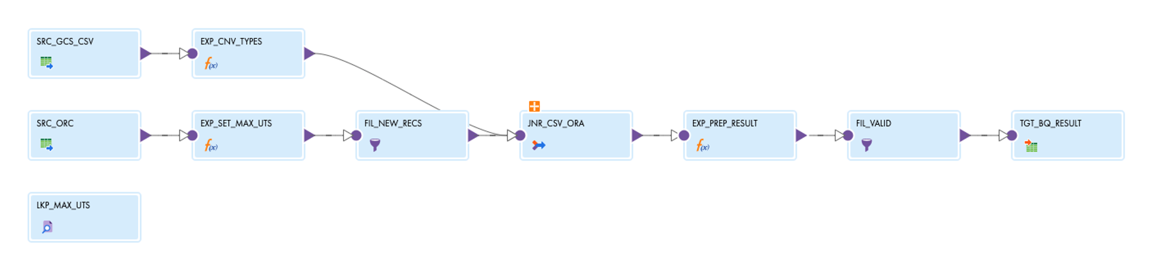
After saving the mapping, it looks like this:
After you have changed a mapping, you have to update the mapping task once so that it retrieves the connection information for all new sources, targets and lookups. To do this, open the TSK_HYBRID_PROTOTYPE task, click on Edit, then on Next and then on Finish.
Step 2: Re-fetch in MetaKraftwerk
To import the changes made to the mapping in Informatica into MetaKraftwerk, we click on the Pattern (again in MetaKraftwerk) and then on  the top right of the bar. Then click on Connect and then simply on 'Fetch 1 Object', our taskflow is already preselected from the last time. After a short time, the resolution interface opens, in which you can specify renaming of mappings, transformations or ports if necessary, but in our case everything fits and we click on Commit.
Since the lookup should go to a different table for each instance, we have to design it dynamically. We open the lookup in the mapping editor in MetaKraftwerk and go to Properties, where we open the property editor by clicking on the property query, then activate 'Advanced Configuraiton'. In the editor, we enter the following expression:
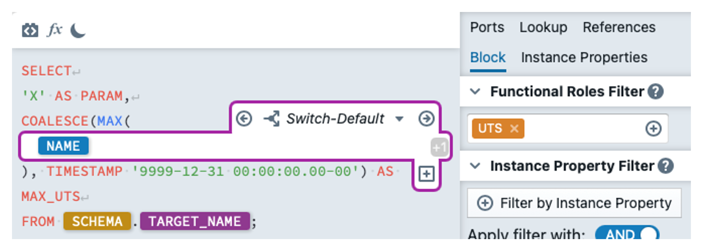
As the update timestamp has a different name in each target table, we must insert an expression block within MAX() with the functional role UTS. In the block, we then specify the instance property NAME so that the name of the UTS is used here.
In the FIL_NEW_RECS filter, we enter the following expression for the filter condition:
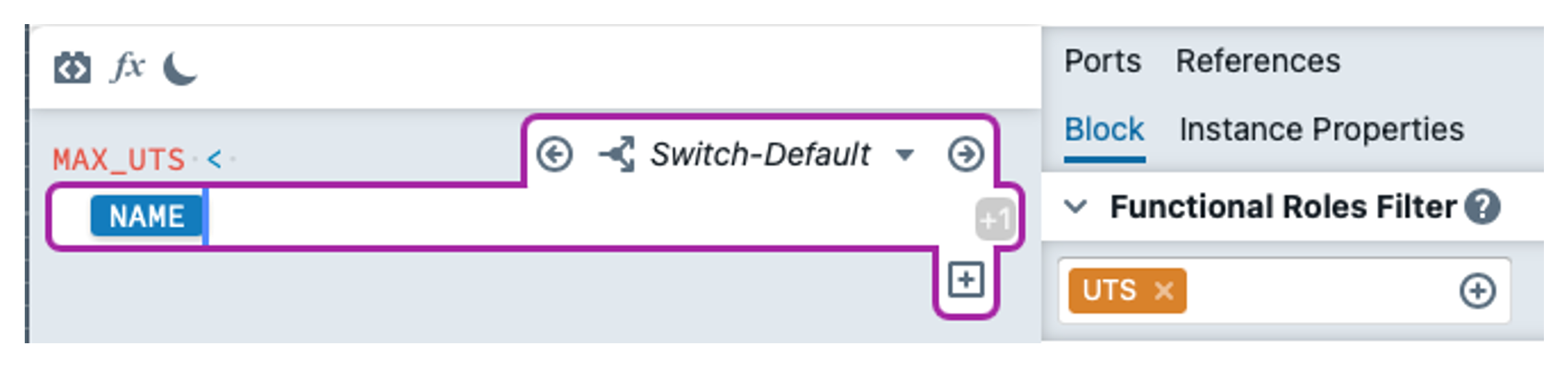
We are finished with the changes.
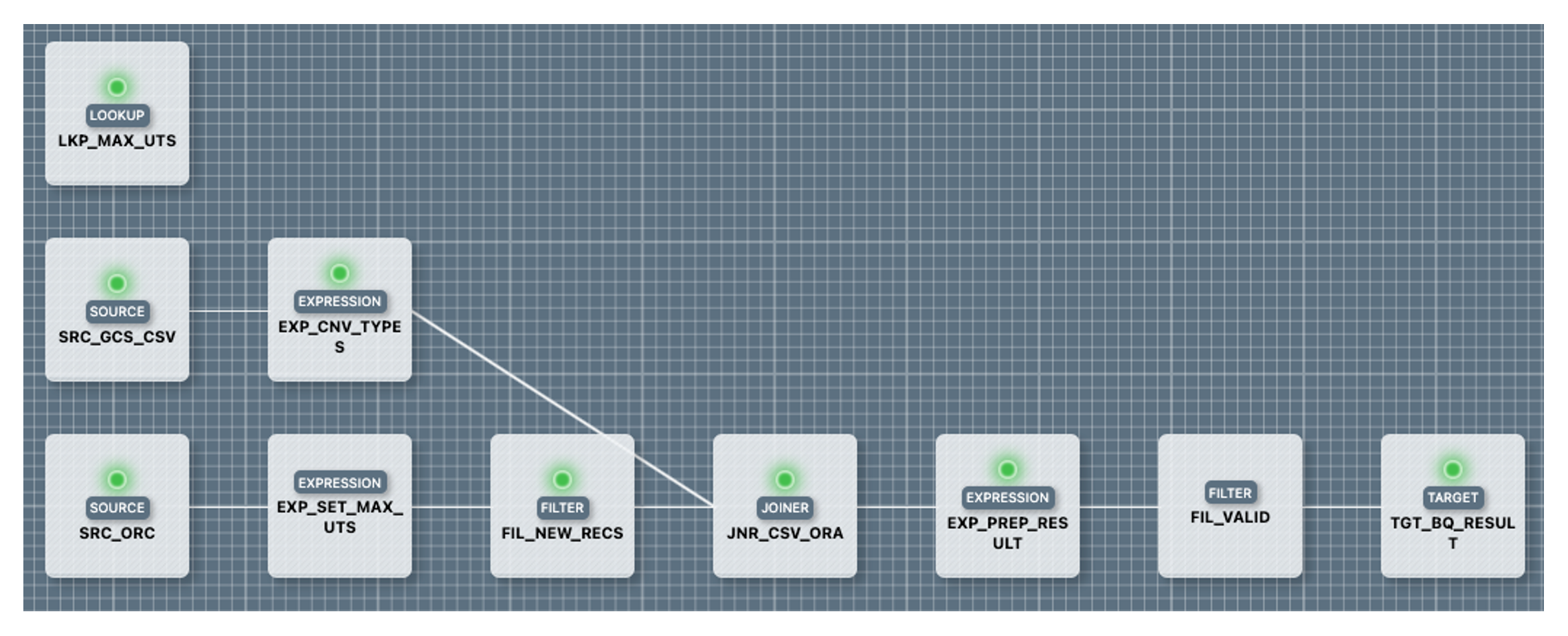
The pattern mapping now looks like the screenshot. The transformations with green lights are dynamically configured in at least one place.
Step 3: Re-deployment of the instances
To deploy the instances with the current functionality, we simply select all instances under Instances and then click on Build again. After a short time, the taskflows are available in Informatica, where they can be restarted. The expectation is that data will be read from the mapping, but no data will be written to the target table. This is because the delta mechanism should retrieve the maximum UTS for the filter from the target table, which in our case is of course the maximum of the previous load.